记录到 MLflow
在我们之前的章节中,我们完成了第一个 MLflow 实验的设置,并为其添加了自定义标签。正如我们很快会发现的,这些标签对于无缝检索属于更广泛项目的相关实验至关重要。
在上一个部分,我们创建了一个数据集,我们将使用它来训练一系列模型。
在本节接下来的内容中,我们将深入探讨 MLflow Tracking 的核心功能
- 利用
start_run上下文来创建和高效管理运行。 - 日志记录的介绍,涵盖标签、参数和指标。
- 理解模型签名的作用和形成。
- 记录一个训练好的模型,巩固其在我们的 MLflow 运行中的存在。
但首先,有一个基础性的步骤等待着我们。对于我们接下来的任务,我们需要一个数据集,专门关注苹果销售。虽然上网搜索很容易,但创建自己的数据集将确保它完美地符合我们的目标。
创建苹果销售数据集
让我们撸起袖子,构建这个数据集。
我们需要一个数据集来定义受周末、促销和价格波动等各种因素影响的苹果销售动态。这个数据集将作为我们预测模型构建和测试的基石。
但在我们开始之前,让我们回顾一下我们到目前为止学到的知识,以及这些原则是如何用于创建本教程的数据集的。
在项目早期开发中使用实验
正如下面的图表所示,我尝试走了许多捷径。为了记录我尝试过的内容,我创建了一个新的 MLflow 实验来记录我尝试的状态。由于我使用了不同的数据集和模型,我尝试的每一次后续修改都需要一个新的实验。

在找到一个可行的合成数据集生成器方法后,结果可以在 MLflow UI 中看到。

一旦我找到了真正有效的方法,我就清理了所有东西(删除了它们)。

如果您正在严格按照本教程进行操作,并且删除了您的 Apple_Models 实验,请在继续教程的下一步之前重新创建它。
使用 MLflow Tracking 来跟踪训练
现在我们有了数据集,并且已经对运行记录方式有了一些了解,让我们深入探讨如何使用 MLflow 来跟踪训练迭代。
首先,我们需要导入所需的模块。
import mlflow
from sklearn.model_selection import train_test_split
from sklearn.ensemble import RandomForestRegressor
from sklearn.metrics import mean_absolute_error, mean_squared_error, r2_score
请注意,这里我们没有直接导入 MlflowClient。对于这部分,我们将使用 fluent API。fluent API 使用 MLflow Tracking 服务器 URI 的全局引用的状态。这个全局实例允许我们使用这些“更高级别”(更简单)的 API 来执行所有可以使用 MlflowClient 完成的操作,并添加了一些其他有用的语法(例如我们很快就会使用的上下文管理器),以尽可能简化将 MLflow 集成到 ML 工作负载中。
为了使用 fluent API,我们需要将全局引用设置为 Tracking 服务器的地址。我们通过以下命令来实现这一点:
mlflow.set_tracking_uri("http://127.0.0.1:8080")
设置好之后,我们可以定义一些我们将用于以运行形式将训练事件记录到 MLflow 的常量。我们将首先定义一个将用于记录运行的实验。当我们需要迭代一些想法并需要比较测试结果时,实验与运行的父子关系及其效用将变得非常清楚。
# Sets the current active experiment to the "Apple_Models" experiment and
# returns the Experiment metadata
apple_experiment = mlflow.set_experiment("Apple_Models")

# Define a run name for this iteration of training.
# If this is not set, a unique name will be auto-generated for your run.
run_name = "apples_rf_test"

# Define an artifact path that the model will be saved to.
artifact_path = "rf_apples"
定义了这些变量后,我们就可以开始实际训练模型了。
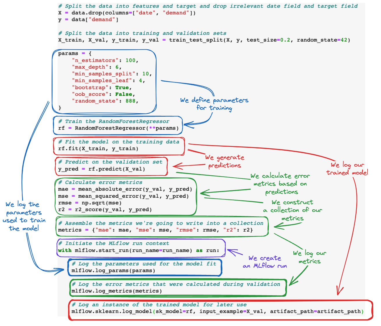
首先,让我们看看我们将要运行什么。在代码显示之后,我们将查看代码的注释版本。
# Split the data into features and target and drop irrelevant date field and target field
X = data.drop(columns=["date", "demand"])
y = data["demand"]

# Split the data into training and validation sets
X_train, X_val, y_train, y_val = train_test_split(X, y, test_size=0.2, random_state=42)

params = {
    "n_estimators": 100,
    "max_depth": 6,
    "min_samples_split": 10,
    "min_samples_leaf": 4,
    "bootstrap": True,
    "oob_score": False,
    "random_state": 888,
}

# Train the RandomForestRegressor
rf = RandomForestRegressor(**params)

# Fit the model on the training data
rf.fit(X_train, y_train)

# Predict on the validation set
y_pred = rf.predict(X_val)

# Calculate error metrics
mae = mean_absolute_error(y_val, y_pred)
mse = mean_squared_error(y_val, y_pred)
rmse = np.sqrt(mse)
r2 = r2_score(y_val, y_pred)

# Assemble the metrics we're going to write into a collection
metrics = {"mae": mae, "mse": mse, "rmse": rmse, "r2": r2}

# Initiate the MLflow run context
with mlflow.start_run(run_name=run_name) as run:
    # Log the parameters used for the model fit
    mlflow.log_params(params)

    # Log the error metrics that were calculated during validation
    mlflow.log_metrics(metrics)

    # Log an instance of the trained model for later use
    mlflow.sklearn.log_model(sk_model=rf, input_example=X_val, name=artifact_path)
为了帮助可视化 MLflow tracking API 调用如何添加到 ML 训练代码库中,请参见下图。
整合在一起
让我们看看当我们运行模型训练代码并导航到 MLflow UI 时会发生什么。

恭喜您完成了 MLflow Tracking 的深度教程!您现在可以 返回“入门” 内容,了解更多关于 MLflow 的信息。
如果您想尝试一些笔记本电脑,以了解 MLflow 如何详细工作,您可以导航到 “入门笔记本电脑”,将示例下载到本地并运行它们!